How to Make Tables in Excel Easy and Practical – Suitable for beginners who are just learning. You can create tables in just a few steps.

How to Make Tables in Excel Easy and Practical
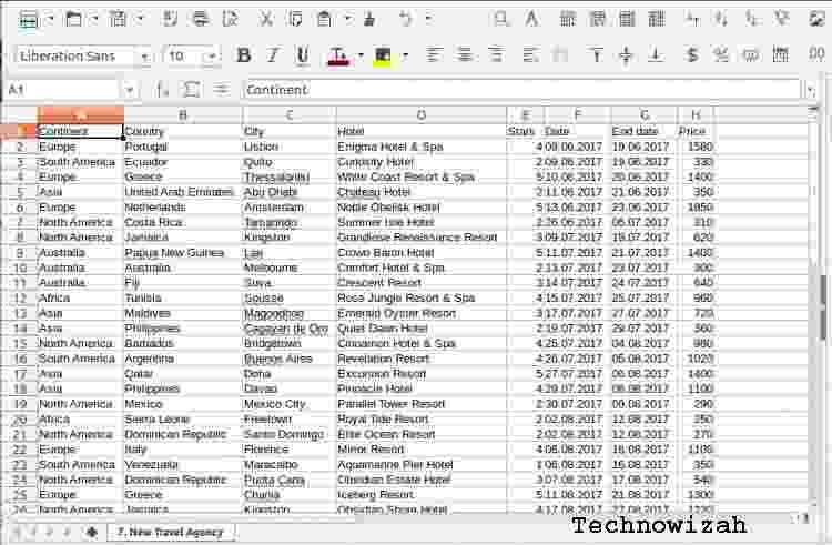
The table is a list that contains data from the summary data. Now, the presence of Excel software makes it easy for us to make it without having to draw.
Read more:
- How to Delete Blank Pages in Microsoft Word
- How to Activate Microsoft Office 2010: 3 Quick Ways
- How to Reinstall Applications on Microsoft Store
- How to Install Apps from Microsoft Store on Windows 10
Curious about how to create a table in Excel? Well, here, we will try to share the ways. How to create a table in Excel 2010, is the same as any other version.
Here, we will explain how to make a table practically. For those of you who want to be good at creating tables in Excel, see this article to the end.
Understanding Excel Tables
The tables that we create in Excel are the same as conventional tables that we make through paper media. We can also make it according to the desired shape. The contents can be text or numbers.
The Excel table itself is a set of columns and rows in a worksheet. It has provided a variety of powerful features and tools.
The function of this feature is to group related data on certain information. Then, the data is formed into a table.
There is also a way to create a table in Excel with formulas. Its function is to make it easier for us to count, add, and the like.
How to Make a Table in Excel
Now, it’s time for the discussion you’ve been waiting for. How to make a table in Excel 2019 that we share, it can also be for other versions. Because basically, it’s still the same. Here are the steps:
Steps to Create a Table in All Versions of Excel
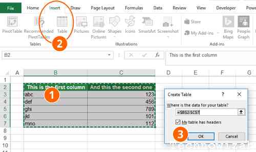
Step 1: Open Excel and Select the Insert Menu
Open the application and double-click the Excel document. Look for the Insert menu then select Table to create a Microsoft Excel document.
Step 2: Click OK in the New Window
If a new window appears, please click the OK button below it. Please check “My table has headers” in the new window if you have cells at the top, then click OK.
Step 3: Choose a Design
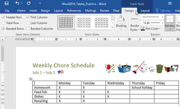
To change the table design, go to the Design tab at the top of the Excel window. Then please select one of the designs in the form of a colored box. It’s located in the “Table Styles” section of the toolbar.
Table Styles Options
You can also modify it via the toolbar called “Table Styles Options” with the following options:
First Column and Last Column: If selected, the contents of the first and last column and header will be in bold.
Banded Columns: Choose this design if you want alternating column colors. If you want to display a uniform column, please uncheck it.
Header Row: Please check this design option, so that the column names are placed in the top cell of the data group.
Banded Rows: This design is for alternating colors in rows. You can also uncheck this design to bring out the lines in a uniform color.
Total Row: Its function is to add a row at the bottom of the table that will show the number of rows of columns on the right.
Filter Button: When selecting it, a drop-down box will be placed at the head of each column. That way, we will easily change the appearance of the data in the column that is created.
After that, please return to the Home tab, then you will return to the Home toolbar. All changes that have been made will not change.
Filtering Data on Table
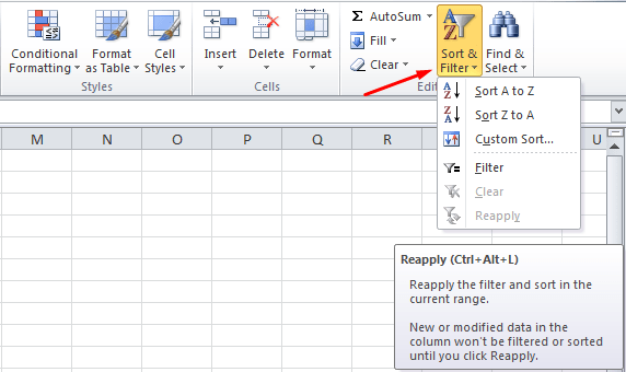
Select or click the drop-down arrow to the right of the data column to filter. After that, a drop-down menu will appear.
Please select a filter on the drop-down menu. There are several menus that you can choose from as follows:
Sort Largest to Smallest: Its function is to sort from the largest to the smallest.
Sort Smallest to Largest: This filter function sorts data from smallest to largest.
Number Filters and Sort by Color: Functions as additional options. You can choose one of them depending on your data needs.
After selecting one, a new window will appear, then just click OK. The filter will then be applied to the table.
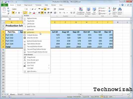
How to Create an Excel Table with Borders
How to create a table in Excel can be applied in version 2007 or another. The method is very easy, even beginners don’t take long to make it. Here we describe the steps:
- The block of data in the Excel column that you will turn into a table.
- Please click the border button which has the Home menu table icon.
- Please select the available border type. If you want to choose to create a full table, please select “All Borders”.
- There are several other features that you can use to customize the table according to your needs.
Examples include font, fill, number, and others. Please select “More Borders” at the bottom to bring up the menu.
- Click OK when the Border settings are complete, and the table is ready.
- You can also edit or modify the border shape. Please enter the Home menu.
Many features can be used to modify, such as Themes Colors for Colors, Fonts, and others.
Advantages of Tables from Excel
Before going into the steps on how to create a table in Excel 2013, and other versions, we will share the following advantages information:
- Tables can be made according to the design and style that we want.
- There are many features to help us in creating a custom table.
- It’s easy when we want to add rows of data without needing to change the table references that we have created.
- Tables can be combined with formulas as needed.
- Can add subtotals and filter buttons automatically.
- To make it easy to remember, we can also add a name.
Read more:
- How to Scan Laptop With Microsoft Defender Antivirus
- 15+ Best and Free Apps from the Microsoft Store
- 7 Ways to Fix USB Device Not Recognized / Unreadable USB
Conclusion:
This is the information about how to create a table in Excel, How, easy right? Excel will make your job easier. Please form a table as needed through the steps above.
![8 Ways to Fix The Hosted Network Couldn’t Be Started in Windows 10 [2026] 8 Ways to Fix The Hosted Network Couldn't Be Started in Windows 10](https://technowizah.com/wp-content/uploads/2021/07/8-Ways-to-Fix-The-Hosted-Network-Couldnt-Be-Started-in-Windows-10.jpg)


